Who are we up against? Reading NASA's PAH database on a laptop
The first post was about a number we computed for benzene. This one is about the competition: the existing predictions that our pipeline will be compared against. Before you can say “our number is better”, you have to write down, precisely and in advance, what the other numbers are. That is what we did this week, and it turned up two surprises.
What the competition is
Astronomers who see infrared light from carbon molecules in space (the “PAHs”, polycyclic aromatic hydrocarbons: flat molecules made of fused benzene-like rings) compare it with a library of computed spectra. The largest such library we know of is NASA’s PAH IR Spectroscopic Database, PAHdb for short. For thousands of molecules it lists the frequencies at which the molecule absorbs infrared light, and how strongly. Frequencies in this field are given in “wavenumbers”, written cm⁻¹; a typical carbon–hydrogen vibration sits near 3000 cm⁻¹, and the differences we care about are a few cm⁻¹.
Those spectra are computed, not measured. The method (a standard way of computing a molecule’s vibrations, called DFT) is fast enough to do thousands of molecules, but it is known to run a little high, so every computed frequency is multiplied by a correction factor slightly below one, a “scale factor”, chosen so that the results match a handful of laboratory spectra. Our project aims to replace that factor, for a subset of molecules, by a correction that is computed with a much more accurate and much slower method, with an error bar. To show that this is worth anything, we must do better than the scaled numbers: not on benzene, where we only want to agree with the laboratory, but on the larger molecules.
So the library is the opponent. Step one of a fair contest: read the opponent’s playbook in full and freeze it, so that nobody can later say “you compared against a convenient version”.
Reading 2.5 million bands
NASA offers the library as a download. You fill in a form (an e-mail address and a promise to cite their papers), and a link arrives. The file is a large structured text file that unpacks to half a gigabyte. A small Python script reads it in a few minutes on a laptop and turns it into two tables: one row per molecule (10,749 of them) and one row per absorption band (2,517,399 of them). Every table records a fingerprint of the file it came from (a checksum), so the version is pinned by its contents, not by its name.
Here is what the molecules look like, sorted by size and electric charge:
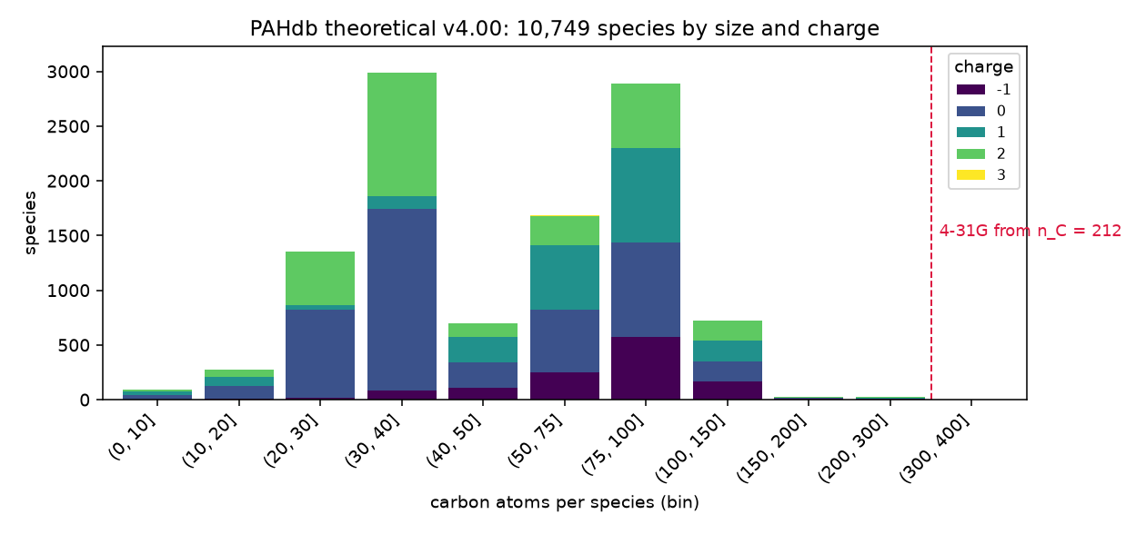
Most of the library lives between 20 and 100 carbon atoms. Above about 200 carbons the computation used a coarser description of the electrons, because the full one becomes too expensive (the red line); there are only 14 molecules up there. Among them is the giant we are eventually aiming at, C₃₈₄H₄₈: 384 carbons and 48 hydrogens, a flat flake of 432 atoms. It is in the library twice, once neutral and once doubly charged, and the neutral one’s 1,290 computed bands look like this:
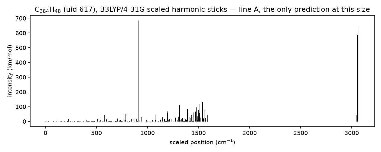
For a molecule of that size, this scaled-DFT spectrum is the only prediction we have found anywhere. That gap is the whole point of the project.
Surprise one: benzene is not in it
Our first test molecule, benzene, does not appear in the library at all: not as a neutral molecule, not as an ion. The smallest entries are a few six- and nine-carbon relatives (phenol, indene and the like); the smallest plain PAH is naphthalene, two rings, ten carbons. On reflection that makes sense. PAHdb is a database of polycyclic molecules, and benzene has only one ring.
For us that is fine, even convenient. Benzene is a calibration molecule in our plan, not a target: it is small enough to compute with our slowest and most accurate method, and its laboratory spectrum is measured to a tenth of a wavenumber. On benzene we only want to agree with the laboratory. That the opponent has no entry there just means the contest starts at naphthalene, where all the competing predictions line up:
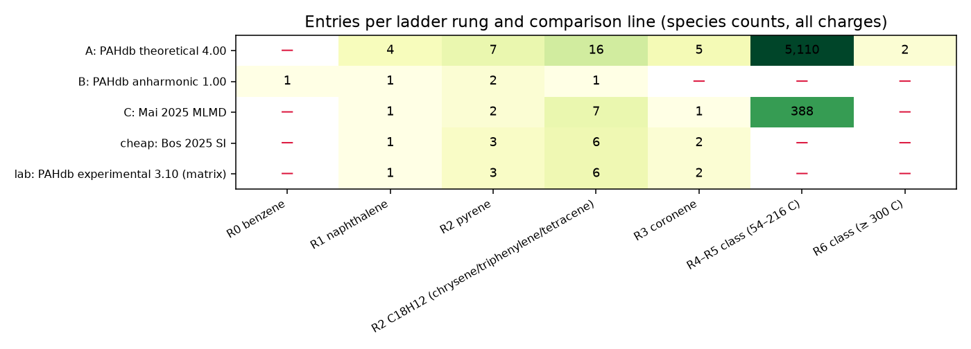
The rows are the four kinds of prediction we compare against: NASA’s scaled library; NASA’s smaller “anharmonic” library, which treats the vibrations as more than perfect springs and covers 45 small molecules; a machine-learning simulation of 1,704 molecules; and a machine-learned scale-factor method. The columns are our sequence of test molecules, from benzene up to the giant flake. A dash means “no prediction exists”. Read along the lower rows and you see how quickly the competition thins out as the molecules get bigger.
Surprise two: the scale factors in the file are not the ones in the paper
This one took an evening to sort out. The paper describing the current library version says the frequencies were scaled by three factors, one per region of the spectrum: 0.964 for the carbon–hydrogen stretching bands near 3000 cm⁻¹, 0.979 for the middle of the spectrum, 0.975 for the low-frequency end. The file stores each band together with the factor that was applied to it. None of the 2.5 million bands carries any of those three numbers. In the same order, from high frequency to low, they carry 0.9597, 0.9691 and 0.9794:
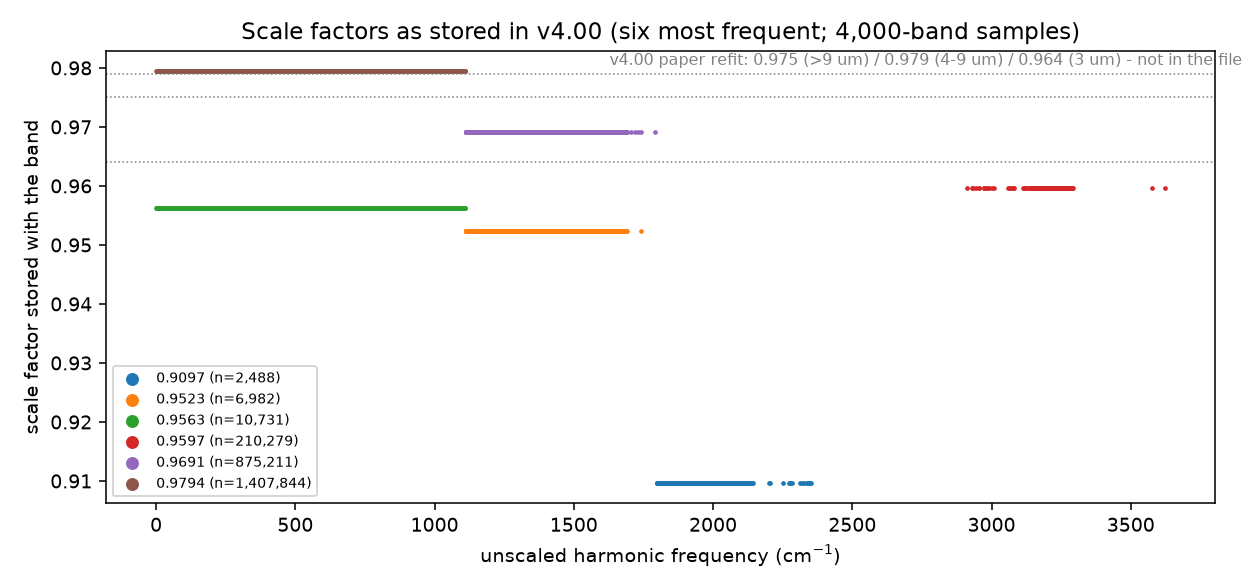
Those three numbers are the factors of the previous library version, published in a table in the 2018 paper. So the file you download today appears to be scaled with the earlier factors, and the new fit described in the current paper does not appear in it. We do not know why: it could be a download that lags the paper, a metadata field that was never updated, or a version mismatch on the website, and we have not asked the database team. We read the stored frequencies as scaled ones because dividing them by the stored factor gives back numbers in the range of raw DFT results (we checked this on naphthalene’s C–H stretch).
The difference is not cosmetic. At a C–H stretching band near 3050 cm⁻¹, the two sets of factors put the band about 13 cm⁻¹ apart; at a band near 1500 cm⁻¹, about 15 cm⁻¹. Those are the same sizes as the improvements we hope to demonstrate.
What do you do with that? You do not pick the version that suits you. We decided to score against the library as served, because that is what every user of the database gets, and because the two other methods in our comparison that build on it, the machine-learning simulation and the scale-factor method, were built on the served file too. Beside it we print a second column with the paper’s factors, labelled, so a reader can see both. The decision is written down with a date, before we have any result of our own.
Why this matters more than it looks
None of this week’s work involved our own pipeline. No new quantum-chemistry calculation, no clever idea. It was reading, parsing, counting, and writing down what we found, with checksums. It is the least glamorous part of a research project and, in my experience so far, the part where the most surprises hide. Two of the “facts” we had carried around since the plan was written turned out to be wrong: that benzene would have a library entry to compare against, and that the library used the factors its paper describes.
Both corrections cost nothing to make now. Either would have been painful to discover after we had numbers of our own, because then every reader would rightly ask whether we had chosen the comparison to flatter ourselves. The rule we follow, freeze the opponent before you have a score, exists for exactly that reason.
Next post: what one naphthalene calculation at our anchor level costs on a laptop, and what that does to the schedule.
Everything in this post comes from the project repository: the parser and tables of Module 02 (commit 61e1ead), the notebook with these figures and the scale-factor reading (commit 8c73aa6), and the dated decision on which factors count (commit 2a2f8da). The library is the public NASA Ames PAH IR Spectroscopic Database, computed library version 4.00; the two papers are Ricca et al. 2026 (ApJS 282, 7) and Bauschlicher et al. 2018 (ApJS 234, 32). The data are computed science data and are the opponent of this project’s pipeline, not its training data.